DISTRIBLAG.RPF

DISTRIBLAG.RPF is an example of estimation of distributed lags and ARDL models. It estimates a distributed lag of long-term interest rate series (composite yield on long-term U.S. Treasury bonds) on a short-term one (yield on 90 day Treasury bills), monthly from 1947:1 to 2007:4. This same data set is used in example files AKAIKE.RPF (lag length choice by information criteria), PDL.RPF (polynomial distributed lags), SHILLER.RPF (Shiller smoothness prior with mixed estimation), and SHILLERGIBBS.RPF (Shiller smoothness prior with Gibbs sampling) to demonstrate various ways to estimate distribute lags.

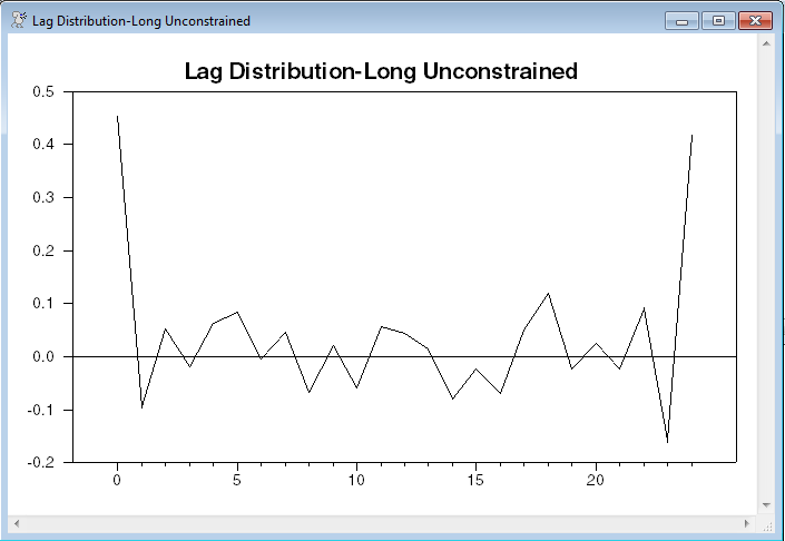
An unrestricted distributed lag from 0 to 24 is done with

linreg longrate
# constant shortrate{0 to 24}

Because of multicollinearity, the individual coefficients in a distributed lag regression usually are poorly determined. For instance, in the unconstrained lag estimate, only the 0 and 24 are (individually) statistically significant at conventional levels. Thus we are interested more in summary measures, in particular, the sum and the shape of the lag distribution. There are several instructions or options which can be very helpful in obtaining this information:

•The instruction SUMMARIZE is designed specifically for computing the sum of a set of lag coefficients.

•The lag coefficients themselves can be extracted from the %BETA vector defined by LINREG.

This uses SUMMARIZE to compute the sum of the full set of lag coefficients. Then lag coefficients are pulled out of the %BETA vector into LAGDIST, using SET. The lag coefficients are in slots 2 through 26 of %BETA, corresponding to lags 0 to 24, in order (slot 1 is the coefficient on the CONSTANT). The NUMBER option on GRAPH causes it to label entry 1 as 0, 2 as 1, etc, thus getting the lag labels correct.

summarize

# shortrate{0 to 24}

set lagdist 1 25 = %beta(t+1)

graph(header="Lag Distribution-Long Unconstrained",number=0)

# lagdist 1 25

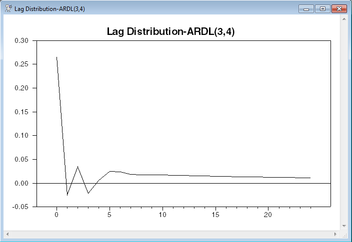
This program next estimates an ARDL(3,4) model (3 autoregressive, current plus 4 l"distributed lag" on the explanatory variable). These were chosen using a preliminary stepwise regression (done with STWISE).

linreg longrate

# constant longrate{1 2 3} shortrate{0 to 4}

The following extract the lag polynomials from the regression. (On the %EQNxxxxx functions, equation “0” is the most recent regression). %EQNLAGPOLY recognizes the LONGRATE is the dependent variable, so it returns in ARPOLY the coefficients for

\begin{equation} 1 - \alpha _1 L - \alpha _2 L^2 - \alpha _3 L^3 \label{eq:linreg_ardldenominator} \end{equation}

while DLPOLY (for the explanatory variable) will be

\begin{equation} \beta _0 + \beta _1 L + \beta _2 L^2 + \beta _3 L^3 + \beta _4 L^4 \label{eq:linreg_ardlnumerator} \end{equation}

Then DLPOLY is divided by ARPOLY and expanded out to the 24th degree.

compute arpoly=%eqnlagpoly(0,longrate)

compute dlpoly=%eqnlagpoly(0,shortrate)

compute ardlpoly=%polydiv(dlpoly,arpoly,24)

The VECTOR information is ARDLPOLY is then copied again into the series LAGDIST and graphed (as with the unrestricted lags, using the NUMBER option to get the lags labeled correctly).

set lagdist 1 25 = ardlpoly(t)

graph(header="Lag Distribution-ARDL(3,4)",number=0)

# lagdist

This computes the long-run response by evaluating the polynomials at the value 1.

disp "LR Response" %polyvalue(dlpoly,1.0)/%polyvalue(arpoly,1.0)

This gives a similar value to the SUMMARIZE on the unrestricted lag (.941 vs .926) and the lag distributions are broadly similar except the unrestricted lag turns up sharply at the final lag. That’s a common feature for long unrestricted lags on data with high serial correlation.

Full Program

open data haversample.rat
calendar(m) 1947
data(format=rats) 1947:1 2007:4 fltg ftb3
set shortrate = ftb3
set longrate = fltg
*
* Long unrestricted lags
*
linreg longrate
# constant shortrate{0 to 24}
summarize
# shortrate{0 to 24}
set lagdist 1 25 = %beta(t+1)
graph(header="Lag Distribution-Long Unconstrained",number=0)
# lagdist 1 25
*
* ARDL estimates
*
linreg longrate
# constant longrate{1 2 3} shortrate{0 to 4}
*
* From the regression, extract the autoregressive polynomial, (which will
* be 1-a(1)L-a(2)L^2-a(3)L^3) since LONGRATE is the dependent variable),
* and the distributed lag polynomial. Divide DLPOLY by ARPOLY and expand
* out to the 24th degree.
*
compute arpoly=%eqnlagpoly(0,longrate)
compute dlpoly=%eqnlagpoly(0,shortrate)
compute ardlpoly=%polydiv(dlpoly,arpoly,24)
*
* Copy the expanded polynomial to the series lagdist and graph it.
*
set lagdist 1 25 = ardlpoly(t)
graph(header="Lag Distribution-ARDL(3,4)",number=0)
# lagdist
*
* Compute the long-run response from the ARDL model
*
disp "LR Response" %polyvalue(dlpoly,1.0)/%polyvalue(arpoly,1.0)

Output

Linear Regression - Estimation by Least Squares

Dependent Variable LONGRATE

Monthly Data From 1949:01 To 2007:04

Usable Observations 700

Degrees of Freedom 674

Centered R^2 0.8951770

R-Bar^2 0.8912889

Uncentered R^2 0.9839108

Mean of Dependent Variable 6.1440571429

Std Error of Dependent Variable 2.6181144800

Standard Error of Estimate 0.8632282458

Sum of Squared Residuals 502.23986490

Regression F(25,674) 230.2354

Significance Level of F 0.0000000

Log Likelihood -877.0561

Durbin-Watson Statistic 0.0896

Variable Coeff Std Error T-Stat Signif

************************************************************************************

1. Constant 1.672475104 0.067473794 24.78703 0.00000000

2. SHORTRATE 0.453439132 0.086136629 5.26418 0.00000019

3. SHORTRATE{1} -0.094668190 0.144896493 -0.65335 0.51375318

4. SHORTRATE{2} 0.052983512 0.152244376 0.34802 0.72793667

5. SHORTRATE{3} -0.018857374 0.153371945 -0.12295 0.90218183

6. SHORTRATE{4} 0.063790400 0.153616599 0.41526 0.67808578

7. SHORTRATE{5} 0.084543569 0.154480458 0.54728 0.58436975

8. SHORTRATE{6} -0.004286232 0.156341085 -0.02742 0.97813613

9. SHORTRATE{7} 0.046222046 0.156782514 0.29482 0.76822497

10. SHORTRATE{8} -0.066795220 0.156624402 -0.42647 0.66990338

11. SHORTRATE{9} 0.020265529 0.153969413 0.13162 0.89532376

12. SHORTRATE{10} -0.058462752 0.150514569 -0.38842 0.69782848

13. SHORTRATE{11} 0.056806104 0.149407094 0.38021 0.70390916

14. SHORTRATE{12} 0.044969624 0.150030177 0.29974 0.76447004

15. SHORTRATE{13} 0.015649051 0.149403284 0.10474 0.91661036

16. SHORTRATE{14} -0.078691033 0.150520030 -0.52279 0.60128912

17. SHORTRATE{15} -0.023182556 0.153947718 -0.15059 0.88034641

18. SHORTRATE{16} -0.068641873 0.156619259 -0.43827 0.66132938

19. SHORTRATE{17} 0.050922524 0.156858591 0.32464 0.74555452

20. SHORTRATE{18} 0.119791197 0.156413095 0.76586 0.44402520

21. SHORTRATE{19} -0.022025194 0.154557282 -0.14251 0.88672368

22. SHORTRATE{20} 0.024980054 0.153787232 0.16243 0.87101391

23. SHORTRATE{21} -0.023470380 0.153579909 -0.15282 0.87858443

24. SHORTRATE{22} 0.090537387 0.152488292 0.59373 0.55288966

25. SHORTRATE{23} -0.157174438 0.145139493 -1.08292 0.27923126

26. SHORTRATE{24} 0.417377352 0.086179819 4.84310 0.00000159

Summary of Linear Combination of Coefficients

SHORTRATE Lag(s) 0 to 24

Value 0.92602224 t-Statistic 75.73293

Standard Error 0.01222747 Signif Level 0.0000000

Linear Regression - Estimation by Least Squares

Dependent Variable LONGRATE

Monthly Data From 1947:05 To 2007:04

Usable Observations 720

Degrees of Freedom 711

Centered R^2 0.9955953

R-Bar^2 0.9955457

Uncentered R^2 0.9992874

Mean of Dependent Variable 6.0392361111

Std Error of Dependent Variable 2.6550307773

Standard Error of Estimate 0.1771979582

Sum of Squared Residuals 22.324771759

Regression F(8,711) 20088.3109

Significance Level of F 0.0000000

Log Likelihood 228.8438

Durbin-Watson Statistic 1.9494

Variable Coeff Std Error T-Stat Signif

************************************************************************************

1. Constant 0.045318501 0.017465957 2.59468 0.00966315

2. LONGRATE{1} 1.257521169 0.037953552 33.13316 0.00000000

3. LONGRATE{2} -0.503413032 0.059296476 -8.48976 0.00000000

4. LONGRATE{3} 0.218241302 0.037502327 5.81941 0.00000001

5. SHORTRATE 0.265113976 0.016690603 15.88403 0.00000000

6. SHORTRATE{1} -0.357960794 0.027514608 -13.00985 0.00000000

7. SHORTRATE{2} 0.198308672 0.030551896 6.49088 0.00000000

8. SHORTRATE{3} -0.133867709 0.028725788 -4.66019 0.00000377

9. SHORTRATE{4} 0.054437369 0.016251196 3.34975 0.00085156

LR Response 0.94145

Graphs