CVMODEL.RPF

CVMODEL.RPF is an example of Structural VAR estimation. It estimates two structural models for the six-variable Canadian VAR used in IMPULSE.RPF as well as several other examples. It demonstrates the use of the CVMODEL and ERRORS instructions.

The first model is a “B” type model which interprets the orthogonal shocks as two real shocks, two financial market shocks and two nominal shocks. The loadings of these shocks onto the innovations produces a highly overidentified model: there are only six free parameters instead of the fifteen for a just identified model.

\begin{equation} \left[ {\begin{array}{*{20}c} {u_u } \\ {u_c } \\ {u_r } \\ {u_x } \\ {u_m } \\ {u_p } \\ \end{array}} \right] = \left[ {\begin{array}{*{20}c} 1 & 0 & {\beta _{uf1} } & 0 & 0 & 0 \\ {\beta _{cr1} } & 1 & {\beta _{cf1} } & 0 & 0 & 0 \\ 0 & 0 & 1 & {\beta _{rf2} } & 0 & 0 \\ 0 & 0 & 0 & 1 & 0 & 0 \\ {\beta _{mr1} } & 0 & 0 & 0 & 1 & {\beta _{mn1} } \\ 0 & 0 & 0 & 0 & 0 & 1 \\ \end{array}} \right]{\kern 1pt} {\kern 1pt} {\kern 1pt} {\kern 1pt} \left[ {\begin{array}{*{20}c} {v_{r1} } \\ {v_{r2} } \\ {v_{f1} } \\ {v_{f2} } \\ {v_{n1} } \\ {v_{n2} } \\ \end{array}} \right] \end{equation}

The second model is also overidentified, with nine parameters. This is an “A” type model, where non-orthogonalized shocks are mapped to orthogonalized ones.

\begin{equation} \left[ {\begin{array}{*{20}c} 1 & 0 & {\gamma _{ur} } & 0 & 0 & 0 \\ {\gamma _{cu} } & 1 & {\gamma _{cu} } & 0 & 0 & 0 \\ 0 & 0 & 1 & {\gamma _{rx} } & 0 & 0 \\ 0 & 0 & 0 & 1 & 0 & 0 \\ 0 & {\gamma _{mc} } & {\gamma _{mr} } & 0 & 1 & {\gamma _{mp} } \\ 0 & {\gamma _{pc} } & {\gamma _{pr} } & 0 & 0 & 1 \\ \end{array}} \right]{\kern 1pt} {\kern 1pt} {\kern 1pt} {\kern 1pt} \left[ {\begin{array}{*{20}c} {u_u } \\ {u_c } \\ {u_r } \\ {u_x } \\ {u_m } \\ {u_p } \\ \end{array}} \right] = \left[ {\begin{array}{*{20}c} {v_u } \\ {v_c } \\ {v_r } \\ {v_x } \\ {v_{_m } } \\ {v_p } \\ \end{array}} \right] \end{equation}

The setup of the basic VAR is the same as for IMPULSE.RPF, though with a slightly different order on the variables. (You can use any listing order for a structural model, through you have to make sure you define the model based upon the order you choose). These are the initial declarations for the first structural VAR. We need a FRML which evaluations to a RECTANGULAR matrix, which needs to be declared before it can be created. We also need to declare the free parameters:

dec frml[rect] bfrml

nonlin uf1 cr1 cf1 rf2 mf1 mm2

In this case, we’re using “descriptive” names for these (for instance, UF1 is for the loading of the F1 shock onto US GDP, CR1 for the loading of R1 onto the Canadian GDP). You could also use positions like B13, B21, etc. The following constructs the FRML describing the structural model. We strongly recommend using one row per line (with the $ continuation) and using spaces or zero padding to make the columns line up. It will save you a lot of time if you have to make changes, or have some problem with the model. In this case, all parameters are initialized to zero, which often works OK for a model like this. The rows correspond to the dependent variables in the order in which you put them into the model, while the columns correspond to your intended shocks.

frml bfrml = ||1.0,0.0,uf1,0.0,0.0,0.0|$

cr1,1.0,cf1,0.0,0.0,0.0|$

0.0,0.0,1.0,rf2,0.0,0.0|$

0.0,0.0,0.0,1.0,0.0,0.0|$

mf1,0.0,0.0,0.0,1.0,mm2|$

0.0,0.0,0.0,0.0,0.0,1.0||

compute uf1=cr1=cf1=rf2=mf1=mm2=pm2=0.0

This is estimated by using the genetic annealing method first, then polishing the estimates with BFGS. (Structural VAR's can have multiple modes, hence the use of the slower, broader search for the PMETHOD).

cvmodel(b=bfrml,method=bfgs,factor=bfactor,$

pmethod=ga,piters=20) %sigma

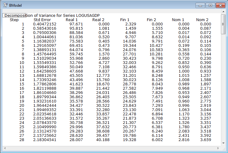
Because the shocks don’t really correspond one-to-one with the variables, the LABELS option is used on ERRORS to give them the desired labels.

errors(model=canmodel,factor=bfactor,steps=28,window="BModel",$

labels=||"Real 1","Real 2","Fin 1","Fin 2","Nom 1","Nom 2"||)

The same procedure is followed with the other model. It just uses the A option on CVMODEL rather than the B option:

dec frml[rect] afrml

nonlin rx ur cu cr pc pr mp mc mr

frml afrml = ||1.0,0.0,ur ,0.0,0.0,0.0|$

cu ,1.0,cr ,0.0,0.0,0.0|$

0.0,0.0,1.0,rx ,0.0,0.0|$

0.0,0.0,0.0,1.0,0.0,0.0|$

0.0,mc ,mr ,0.0,1.0,mp |$

0.0,pc ,pr ,0.0,0.0,1.0||

compute ur=cu=cr=rx=mc=mr=mp=pc=pr=0.0

cvmodel(a=afrml,method=bfgs,factor=afactor,$

pmethod=ga,piters=20) %sigma

errors(model=canmodel,factor=afactor,steps=28,window="AModel")

Full Program

open data oecdsample.rat

calendar(q) 1981

data(format=rats) 1981:1 2006:4 can3mthpcp canexpgdpchs $

canexpgdpds canm1s canusxsr usaexpgdpch

set logcangdp = 100.0*log(canexpgdpchs)

set logcandefl = 100.0*log(canexpgdpds)

set logcanm1 = 100.0*log(canm1s)

set logusagdp = 100.0*log(usaexpgdpch)

set logexrate = 100.0*log(canusxsr)

system(model=canmodel)

variables logusagdp logcangdp can3mthpcp logexrate logcandefl logcanm1

lags 1 to 4

det constant

end(system)

estimate(noprint)

dec frml[rect] bfrml

nonlin uf1 cr1 cf1 rf2 mf1 mm2

frml bfrml = ||1.0,0.0,uf1,0.0,0.0,0.0|$

cr1,1.0,cf1,0.0,0.0,0.0|$

0.0,0.0,1.0,rf2,0.0,0.0|$

0.0,0.0,0.0,1.0,0.0,0.0|$

mf1,0.0,0.0,0.0,1.0,mm2|$

0.0,0.0,0.0,0.0,0.0,1.0||

compute uf1=cr1=cf1=rf2=mf1=mm2=pm2=0.0

* This is estimated by using the genetic method first, then polishing the

* estimates with bfgs. In practice, you might want to repeat this

* several times to test whether there are global identification problems.

cvmodel(b=bfrml,method=bfgs,factor=bfactor,$

pmethod=ga,piters=20) %sigma

* Because the shocks don't really correspond one-to-one with the

* variables, the labels option is used on ERRORS to give them the

* desired labels.

errors(model=canmodel,factor=bfactor,steps=28,window="BModel",$

labels=||"Real 1","Real 2","Fin 1","Fin 2","Nom 1","Nom 2"||)

dec frml[rect] afrml

nonlin rx ur cu cr pc pr mp mc mr

frml afrml = ||1.0,0.0,ur ,0.0,0.0,0.0|$

cu ,1.0,cr ,0.0,0.0,0.0|$

0.0,0.0,1.0,rx ,0.0,0.0|$

0.0,0.0,0.0,1.0,0.0,0.0|$

0.0,mc ,mr ,0.0,1.0,mp |$

0.0,pc ,pr ,0.0,0.0,1.0||

compute ur=cu=cr=rx=mc=mr=mp=pc=pr=0.0

cvmodel(a=afrml,method=bfgs,factor=afactor,$

pmethod=ga,piters=20) %sigma

errors(model=canmodel,factor=afactor,steps=28,window="AModel")

Output

Covariance Model-Concentrated Likelihood - Estimation by BFGS

Convergence in 14 Iterations. Final criterion was 0.0000004 <= 0.0000100

Observations 100

Log Likelihood -585.4719

Log Likelihood Unrestricted -578.6729

Chi-Squared(9) 13.5981

Significance Level 0.1373572

Variable Coeff Std Error T-Stat Signif

************************************************************************************

1. UF1 0.102630163 0.070065484 1.46477 0.14298234

2. CR1 0.500515182 0.104290402 4.79924 0.00000159

3. CF1 -0.077813852 0.079754083 -0.97567 0.32922687

4. RF2 -0.084722322 0.036190823 -2.34099 0.01923273

5. MF1 -0.161403447 0.108387565 -1.48913 0.13645248

6. MM2 0.112152267 0.042611628 2.63196 0.00848929

Covariance Model-Concentrated Likelihood - Estimation by BFGS

Convergence in 18 Iterations. Final criterion was 0.0000028 <= 0.0000100

Observations 100

Log Likelihood -581.0251

Log Likelihood Unrestricted -578.6729

Chi-Squared(6) 4.7044

Significance Level 0.5822397

Variable Coeff Std Error T-Stat Signif

************************************************************************************

1. RX 0.096444096 0.036861996 2.61636 0.00888739

2. UR -0.099391995 0.072913270 -1.36315 0.17283407

3. CU -0.504941212 0.104916628 -4.81279 0.00000149

4. CR 0.146654170 0.078837808 1.86020 0.06285709

5. PC -0.226893636 0.227477992 -0.99743 0.31855528

6. PR 0.306165446 0.165721688 1.84747 0.06467940

7. MP -0.121270363 0.048212171 -2.51535 0.01189151

8. MC 0.204902146 0.105038542 1.95073 0.05108882

9. MR 0.040661738 0.086947863 0.46766 0.64003022

Reports

This generates two rather lengthy reports with the error decompositions from the two models. Below is part of one of those (for the second "B" model).