UNION.RPF

UNION.RPF is an example of estimation of probit, logit and linear probability models. This is adapted from Johnston and DiNardo(1997), pp 415-425. It analyzes the probability of union membership using a sample of 1000 individuals.

This first does a comparison of basic statistics for subsamples of union members and non-union members:

table(smpl=union,title="Statistics for Union Members") / $
potexp exp2 grade married high
table(smpl=.not.union,title="Statistics for Non-Union Members") / $
potexp exp2 grade married high

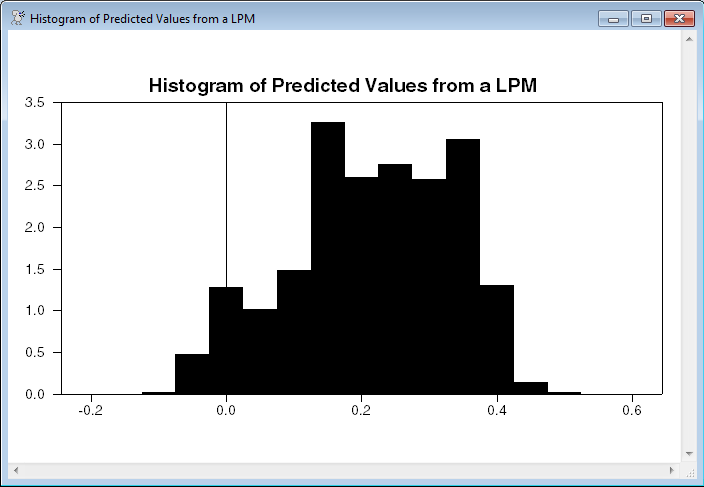
This fits a linear probability model and does a histogram of the predicted “probabilities”. (An LPM doesn't constrain the predictions to the $[0,1]$ range.) DENSITY with the option HISTOGRAM handles the counts for the histogram.

linreg union

# potexp exp2 grade married high constant

prj fitlp

density(type=histogram) fitlp / gx fx

scatter(style=bargraph,$

header="Histogram of Predicted Values from a LPM")

# gx fx

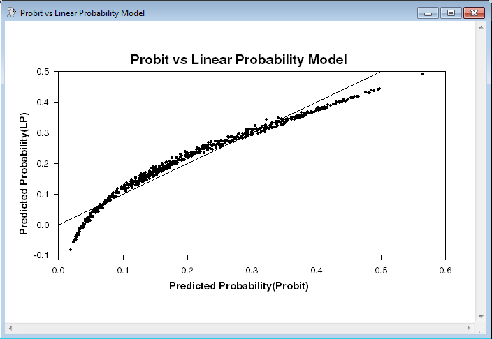
DDV estimates a probit model and shows a scatter graph of the predicted probabilities of the probit (computed using PRJ using the results of the probit estimation) vs. the LPM. The LINES=||0.0,1.0|| option on SCATTER puts a 45 degree line on the graph.

ddv(dist=probit) union

# potexp exp2 grade married high constant

prj(dist=probit,cdf=fitprb)

scatter(style=dots,lines=||0.0,1.0||,$

header="Probit vs Linear Probability Model",$

hlabel="Predicted Probability(Probit)",$

vlabel="Predicted Probability(LP)")

# fitprb fitlp

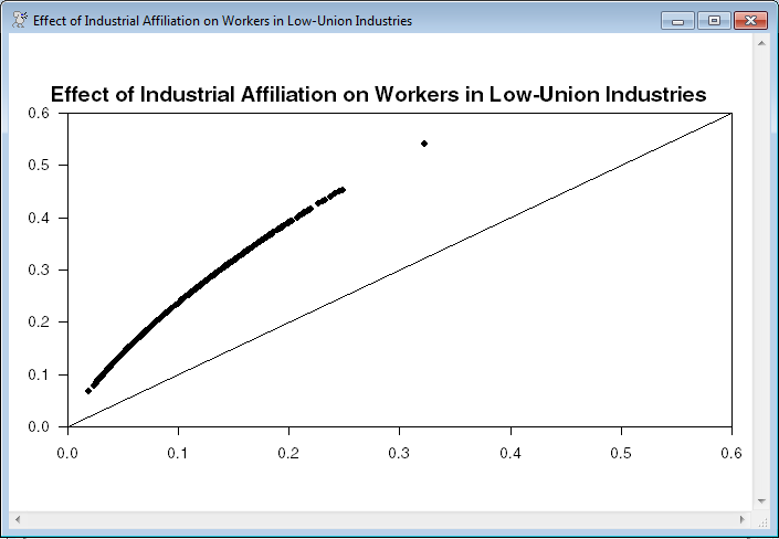
This evaluates the predicted effect of switching industries on individuals currently in low union industries. This is done by evaluating the predicted probabilities with the value of “high” turned on for all the individuals, then knocking out of the sample those who were already in a high union industry. The predicted probabilities are obtained by “dotting” the coefficients with the required set of variables, then evaluating the normal CDF (%CDF) at those values.

set z = %dot(%beta,||potexp,exp2,grade,married,1,1||)

set highprb = %if(high,%na,%cdf(z))

scatter(style=dots,vmin=0.0,lines=||0.0,1.0||,header=$

"Effect of Affiliation on Workers in Low-Union Industries")

# fitprb highprb

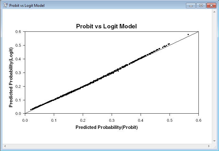
This re-estimates the model using logit rather than probit, and does a scatter graph comparing the probit and logit probabilities.

ddv(dist=logit) union

# potexp exp2 grade married high constant

prj(dist=logit,cdf=fitlgt)

scatter(style=dots,lines=||0.0,1.0||,$

header="Probit vs Logit Model",$

hlabel="Predicted Probability(Probit)",$

vlabel="Predicted Probability(Logit)")

# fitprb fitlgt

Full Program

open data cps88.asc

data(format=prn,org=columns) 1 1000 age exp2 grade ind1 married $

lnwage occ1 partt potexp union weight high

table(smpl=union,title="Statistics for Union Members") / $

potexp exp2 grade married high

table(smpl=.not.union,title="Statistics for Non-Union Members") / $

potexp exp2 grade married high

* Fit a linear probability model. Do a histogram of the predicted

* "probabilities".

linreg(title="Linear Probability Model") union

# potexp exp2 grade married high constant

prj fitlp

density(type=histogram) fitlp / gx fx

scatter(style=bargraph,header="Histogram of Predicted Values from a LPM")

# gx fx

* Probit model. Show a scatter graph of the predicted probabilites of

* the probit vs the LPM. Include the 45 degree line on the graph.

ddv(dist=probit) union

# potexp exp2 grade married high constant

prj(dist=probit,cdf=fitprb)

scatter(style=dots,lines=||0.0,1.0||,$

header="Probit vs Linear Probability Model",$

hlabel="Predicted Probability(Probit)",$

vlabel="Predicted Probability(LP)")

# fitprb fitlp

* Evaluate the predicted effect of switching industries on individuals

* currently in low union industries. This is done by evaluating the

* predicted probabilities with the value of "high" turned on for all the

* individuals, then knocking out of the sample those who were already in

* a high union industry. The predicted probabilities are obtained by

* "dotting" the coefficients with the required set of variables, then

* evaluating the normal cdf (%cdf) at those values.

set z = %dot(%beta,||potexp,exp2,grade,married,1,1||)

set highprb = %if(high,%na,%cdf(z))

scatter(style=dots,vmin=0.0,lines=||0.0,1.0||,$

header="Effect of Industrial Affiliation on Workers in Low-Union Industries")

# fitprb highprb

* Logit model

ddv(dist=logit) union

# potexp exp2 grade married high constant

prj(dist=logit,cdf=fitlgt)

scatter(style=dots,lines=||0.0,1.0||,$

header="Probit vs Logit Model",$

hlabel="Predicted Probability(Probit)",$

vlabel="Predicted Probability(Logit)")

# fitprb fitlgt

Output

Statistics for Union Members

Series Obs Mean Std Error Minimum Maximum

POTEXP 216 22.77777778 11.41710942 1.00000000 49.00000000

EXP2 216 648.57407407 563.34258574 1.00000000 2401.00000000

GRADE 216 12.56018519 2.27342339 5.00000000 18.00000000

MARRIED 216 0.75000000 0.43401854 0.00000000 1.00000000

HIGH 216 0.76388889 0.42567775 0.00000000 1.00000000

Statistics for Non-Union Members

Series Obs Mean Std Error Minimum Maximum

POTEXP 784 17.81122449 12.93830834 1.00000000 55.00000000

EXP2 784 484.42602041 595.76310328 1.00000000 3025.00000000

GRADE 784 13.13903061 2.67619124 0.00000000 18.00000000

MARRIED 784 0.61096939 0.48784152 0.00000000 1.00000000

HIGH 784 0.51403061 0.50012216 0.00000000 1.00000000

Linear Regression - Estimation by Linear Probability Model

Dependent Variable UNION

Usable Observations 1000

Degrees of Freedom 994

Centered R^2 0.0837275

R-Bar^2 0.0791185

Uncentered R^2 0.2816424

Mean of Dependent Variable 0.2160000000

Std Error of Dependent Variable 0.4117201884

Standard Error of Estimate 0.3950972711

Sum of Squared Residuals 155.16524249

Regression F(5,994) 18.1660

Significance Level of F 0.0000000

Log Likelihood -487.3062

Durbin-Watson Statistic 2.0015

Variable Coeff Std Error T-Stat Signif

************************************************************************************

1. POTEXP 0.020038767 0.003896914 5.14221 0.00000033

2. EXP2 -0.000370581 0.000081883 -4.52572 0.00000675

3. GRADE -0.012463581 0.005100452 -2.44362 0.01471364

4. MARRIED 0.013342779 0.030000989 0.44474 0.65660113

5. HIGH 0.143939577 0.025678520 5.60545 0.00000003

6. Constant 0.102136788 0.074933713 1.36303 0.17318220

Binary Probit - Estimation by Newton-Raphson

Convergence in 5 Iterations. Final criterion was 0.0000006 <= 0.0000100

Dependent Variable UNION

Usable Observations 1000

Degrees of Freedom 994

Log Likelihood -475.2514

Average Likelihood 0.6217287

Pseudo-R^2 0.0929077

Log Likelihood(Base) -521.7985

LR Test of Coefficients(5) 93.0941

Significance Level of LR 0.0000000

Variable Coeff Std Error T-Stat Signif

************************************************************************************

1. POTEXP 0.083509133 0.015608799 5.35013 0.00000009

2. EXP2 -0.001530796 0.000317877 -4.81569 0.00000147

3. GRADE -0.042077965 0.018908978 -2.22529 0.02606175

4. MARRIED 0.062251606 0.112583951 0.55293 0.58030792

5. HIGH 0.561295261 0.099662392 5.63197 0.00000002

6. Constant -1.468412409 0.295812594 -4.96400 0.00000069

Binary Logit - Estimation by Newton-Raphson

Convergence in 6 Iterations. Final criterion was 0.0000000 <= 0.0000100

Dependent Variable UNION

Usable Observations 1000

Degrees of Freedom 994

Log Likelihood -475.5541

Average Likelihood 0.6215406

Pseudo-R^2 0.0923048

Log Likelihood(Base) -521.7985

LR Test of Coefficients(5) 92.4887

Significance Level of LR 0.0000000

Variable Coeff Std Error T-Stat Signif

************************************************************************************

1. POTEXP 0.147402074 0.028097014 5.24618 0.00000016

2. EXP2 -0.002686919 0.000565428 -4.75201 0.00000201

3. GRADE -0.070320887 0.032142049 -2.18782 0.02868301

4. MARRIED 0.115463002 0.196778961 0.58676 0.55736156

5. HIGH 0.980141109 0.180049032 5.44375 0.00000005

6. Constant -2.581435857 0.518685883 -4.97688 0.00000065

Graphs