DLMEXAM1.RPF

DLMEXAM1.RPF is a simple example of Kalman smoothing. This uses the model for Nile river flow data common to the four simple DLM examples.

It does Kalman smoothing over the full sample (thus the / for the range). The states are saved into the SERIES[VECT] XSTATES and the covariances into the SERIES[SYMM] VSTATES.

dlm(a=1.0,c=1.0,sv=15099.0,sw=1469.1,y=nile,presample=diffuse,$
type=smooth) / xstates vstates

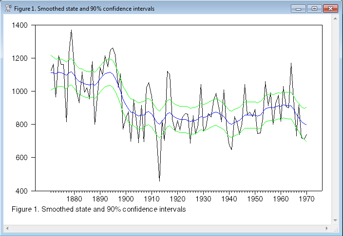
The smoothed means for the underlying level are extracted into the series A and the variances into P. LOWER and UPPER are the lower and upper bounds of a 90% confidence interval.

set a = %scalar(xstates)
set p = %scalar(vstates)
set lower = a+sqrt(p)*%invnormal(.05)
set upper = a+sqrt(p)*%invnormal(.95)

The mean level and actual data are then graphed with a 90% confidence interval.

Full Program

open data nile.dat
calendar 1871
data(format=free,org=columns,skips=1) 1871:1 1970:1 nile
*
dlm(a=1.0,c=1.0,sv=15099.0,sw=1469.1,y=nile,presample=diffuse,$
type=smooth) / xstates vstates
set a = %scalar(xstates)
set p = %scalar(vstates)
set lower = a+sqrt(p)*%invnormal(.05)
set upper = a+sqrt(p)*%invnormal(.95)
*
graph(footer=$
"Figure 1. Smoothed state and 90% confidence intervals") 4
# nile
# a
# lower / 3
# upper / 3

Graph