@ClassicalDecomp does a classical decomposition of the series "x" into a trend-cycle, seasonal and irregular. The seasonals are assumed to be constant across the data range (unlike the moving seasonals done by X11).

 

With SEASONAL=ADDITIVE (the default), the seasonal factors sum to zero, and the data are assumed to take the form

 

\(X = TC + S + I\)

 

With SEASONAL=MULTIPLICATIVE, the seasonal factors are scaled to average 1.0 and the data are assumed to take the form

 

\(X = TC \times S \times I\)

 

The TREND option determines how the final trend-cycle is estimated after the seasonal factors have been computed. LINEAR and QUADRATIC request regressions with 1, \(t\) or 1, \(t\) and \(t^2\) respectively. The default (TREND=MA) does a moving average with correction for end terms.

 

@ClassicalDecomp( options )  x  start end

Parameters

Options

SEASONAL=[ADDITIVE]/MULTIPLICATIVE

TREND=NONE/LINEAR/QUADRATIC/[MA]

These are described above.

 

SPAN=seasonal span [CALENDAR seasonal]

 

TC=(output) estimated trend cycle

FACTORS=(output) estimated seasonal factors

IRREG=(output) estimated irregular component

Example

This does the decomposition of a series of accidental deaths. The raw data have a strong seasonal which we want to remove. The underlying trend is assumed to be a quadratic in time (TREND=QUADRATIC).  The deasonalized data is the combination of the trend and the irregular—because this is an additive model, the seasonal can be removed from the raw data by subtracting it. (If this were SEASONAL=MULTIPLICATIVE, you would divide by the factors). You don't need to extract the trend or irregular since the deseasonalized data can be obtained as the residual from subtracting out the seasonal.

 

*

* Brockwell & Davis, Introduction to Time Series and Forecasting, 2nd ed.

* Example 1.5.4 from page 32

*

open data deaths.dat

calendar(m) 1973

data(format=free,org=columns) 1973:1 1978:12 deaths

*

* @ClassicalDecomp has options SPAN for the seasonal span (here not

* necessary, since the data have already been declared to be monthly),

* TREND=NONE/LINEAR/QUADRATIC to choose the type of trend, and FACTORS

* to get as a return the seasonal component.

*

@ClassicalDecomp(trend=quadratic,factors=s) deaths

set deseas = deaths-s

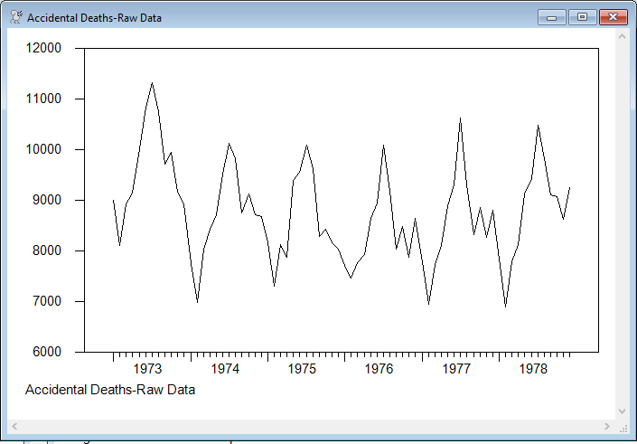
graph(footer="Accidental Deaths-Raw Data")

# deaths

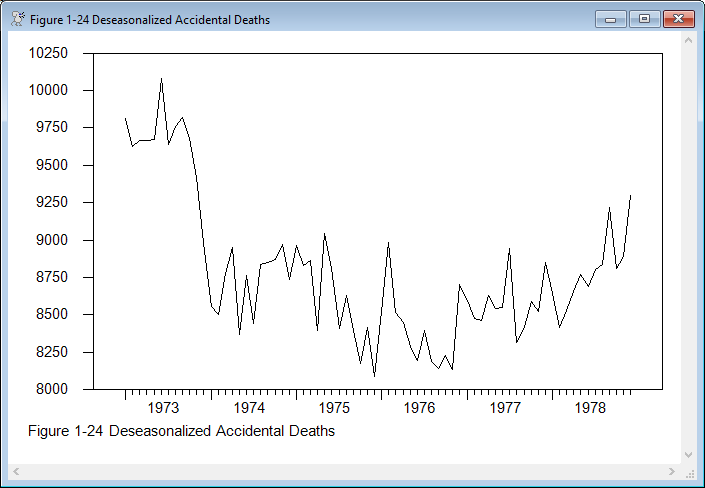
graph(footer="Figure 1-24 Deseasonalized Accidental Deaths")

# deseas

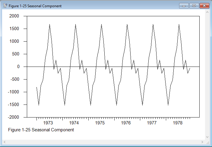
graph(footer="Figure 1-25 Seasonal Component")

# s

Output

The output from the procedure is in the form of three series, with the options TC for the trend-cycle, FACTORS for the seasonal factors and IRREG for the irregular. The raw data are show in the first graph, and they are dominated by the seasonal. The second graph shows the series with the seasonal removed, and the third is the seasonal itself.

 

 

 

 

 

 

Copyright © 2026 Thomas A. Doan